MATH 1040 - Introduction to Statistics

17.1 Sampling Distributions

Outline

Up to this point in the course, we have learned about samples.

Segment 1: Variables, Sampling Methods, Study Design, Graphing
Segment 2: Analysis of Quantitative Variables
Segment 3: Analysis of Categorical Variables using Probabilities

In lesson 15, we learned about Normal Distributions. This will be a critical tool moving forward. In lesson 17, we are going to use normal distributions to learn about the crux of statistics: the Central Limit Theorem.

Imagine you are doing a study on the average height of American females, which is 5 feet 3.5 inches (this would be a population mean).

If you were to randomly select one woman, the chance of her height being near 5 feet 3.5 inches (the population mean) is pretty high. The chance of her height being over 6 feet is low. Not really low, but definitely less probable than a height near the population mean.

Now, if you instead randomly select 4 women, the chances of their mean height (the sample mean) being 6 feet tall or higher is quite low.

Randomly selecting 10 women whose sample mean height is over 6 feet tall is so extremely small it is nearly impossible.

Larger samples lead to lower probabilities that the sample mean is an extreme value, and more likely that the sample mean is near the population mean.

This is the principle of the Central Limit Theorem. If we can create sample large enough, then our sample can more accurately approximate the population. In Lesson 17, we will study more about how the Central Limit Theorem works, then begin implementing it in lessons 18 and 19.

Reading

Lesson

When we learned about probabilities, we started by looking at the probability of a single event (like rolling a die). We introduced the probability of multiple events when we discussed the binomial distributions in lessons 13 and 14. We are not going into binomial distributions right now, but we are going to continue looking at multiple events (like rolling 2 dice).

Here is a graph showing the uniform distribution of rolling 1 die.

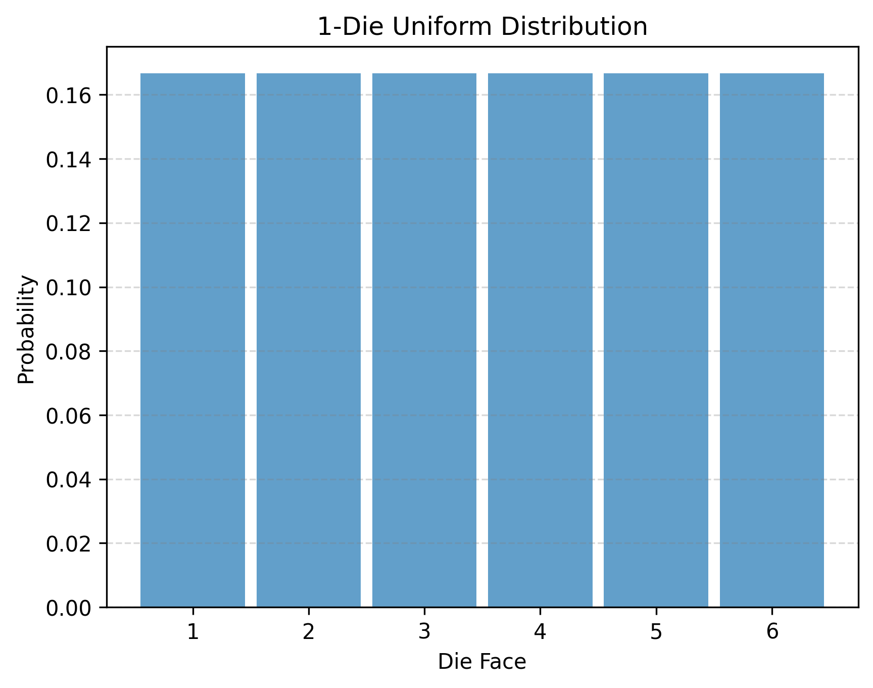
Uniform probability distribution of rolling 1 die

This is the distribution of the population, and it has an expected value (or population mean) of 3.5 (the value right in the middle of the distribution). If we were to simply take a sample (roll a die), we would get something similar but not exact. (We saw this with the Law of Large Numbers back in Lesson 9.)

Sampling Distribution of rolling 1 die 10 times, 100 times, and 1000 times

Let’s instead roll 2 dice and take their average. Here is a table showing the different possible averages of two dice and the possible ways to roll them. Notice the distribution - it looks more normal. This will become important in lesson 17.2.

Mean	1	1.5	2	2.5	3	3.5	4	4.5	5	5.5	6
Possible Rolls	(1,1)	(2,1) (1,2)	(3,1) (2,2) (1,3)	(4,1) (3,2) (2,3) (1,4)	(5,1) (4,2) (3,3) (2,4) (1,5)	(6,1) (5,2) (4,3) (3,4) (2,5) (1,6)	(6,2) (5,3) (4,4) (3,5) (6,2)	(6,3) (5,4) (4,5) (3,6)	(6,4) (5,5) (4,6)	(6,5) (5,6)	(6,6)
Probability	1/36	2/36	3/36	4/36	5/36	6/36	5/36	4/36	3/36	2/36	1/36

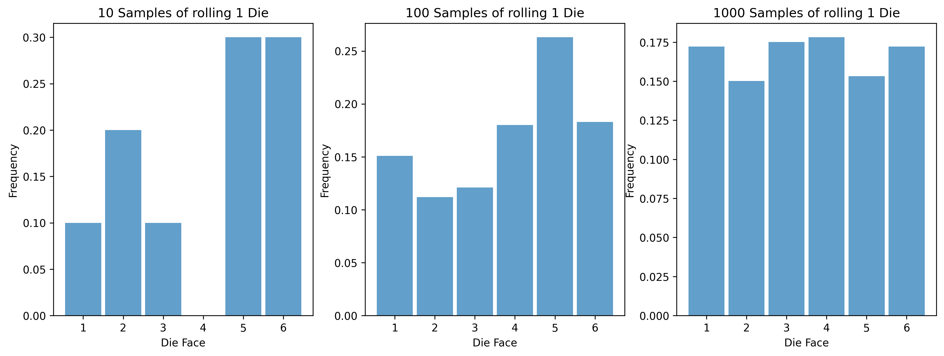
Now, let’s say that I roll 2 dice 10 times, 100 times, then 1000 times. This is the distribution that I get for each.

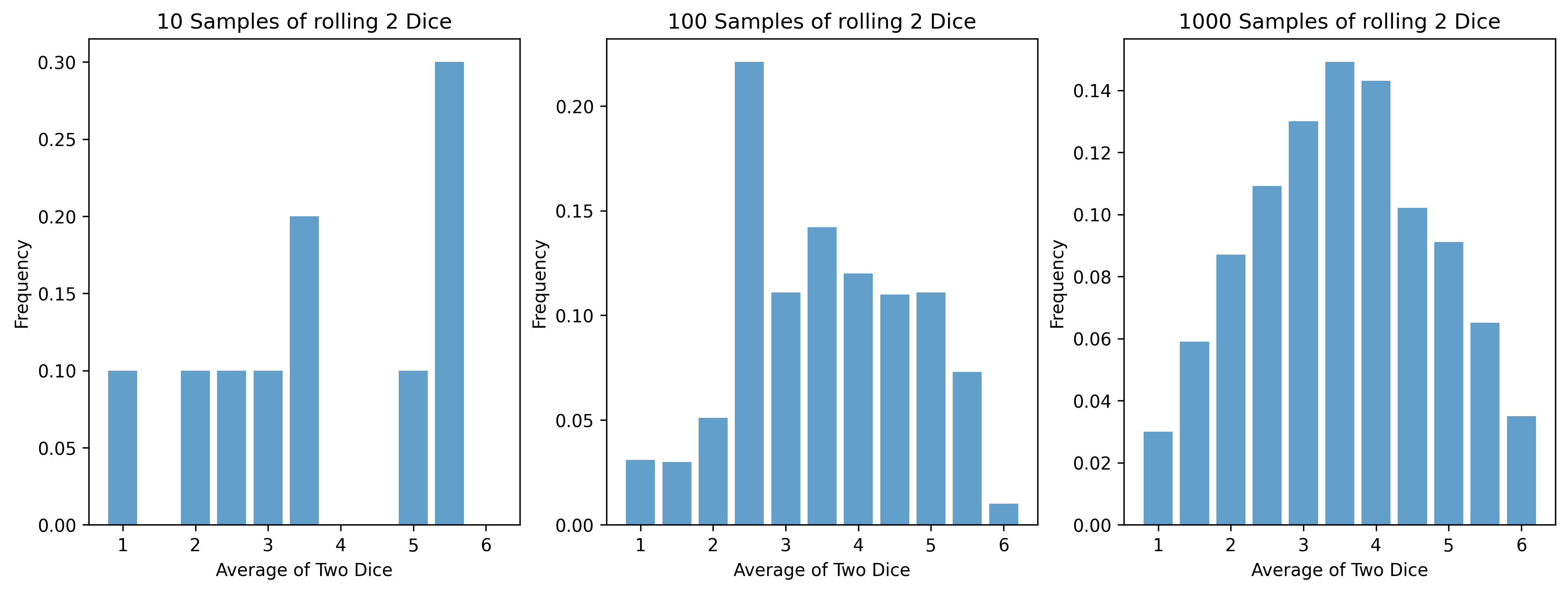
Sampling Distribution of rolling 2 dice 10 times, 100 times, and 1000 times

The Point

Instead of taking 1 sample, we took 2 samples and found the mean. Then we did this over and over and over and found the distribution of these mean values. This is known as a sampling distribution.

What happens with larger samples?

We saw what happens with a sample of 2 dice. What happens if we get a sampling distribution with 10 dice? with 20 dice? with 30 dice? with 50 dice? with more?

The following graph shows what it looks like with larger sample sizes. The blue bars show the histograms from sampling (rolling) with 2 dice, 5 dice, 10 dice, 20 dice, 30 dice, and 50 dice. The red lines show the normal distributions using the mean and standard deviation of our samples.

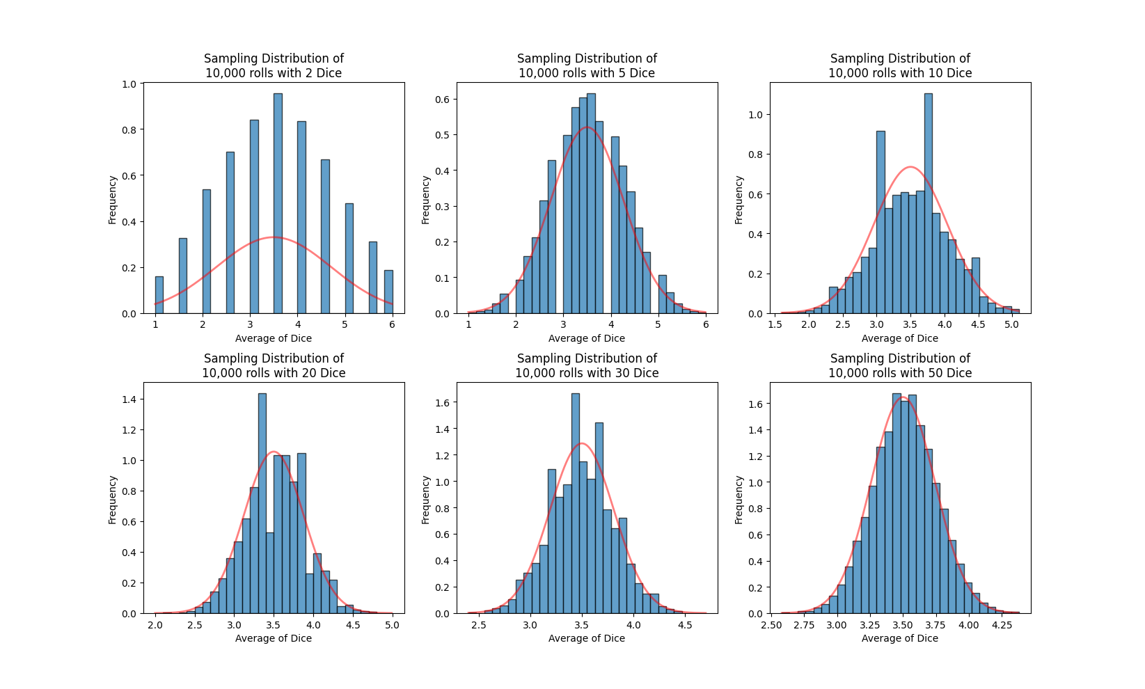
Sampling distribution with sample sizes of 2, 5, 10, 20, 30, and 50

At first, the shape of the distribution is very angular. As the sample size increases, the shape gets closer and closer to the normal distribution. By the time the sample size is 20 or 30, the sampling distribution is normal.

If the sample size is large enough, the sampling distribution becomes normal. As a result, we can use normal distribution mathematics to relate the sample back to the population. This is the first key to the Central Limit Theorem.