MATH 1040 - Introduction to Statistics

Lesson 17.3 The Central Limit Theorem

Reading

Reading sections are from the Introductory Statistics Textbook

• 4.2.2 Examining the Central Limit Theorem
• 4.2.3 Normal approximation for the sampling distribution of $\bar{x}$

Lesson

Examples of using the Central Limit Theorem

At this point, we can use our normal distribution to calculate probabilities as we did in Lessons 15 and 16.

You administer a specialized Competency Exam. The exam takes an average of 45 minutes to complete with a standard deviation of 12 minutes.

You are asked to administer the exam in an area that you suspect will complete the exam in less than 42 minutes.

• What is the probability that one single student completes the exam in less than 42 minutes?

\[\mu = 45 \qquad \sigma = 12\]

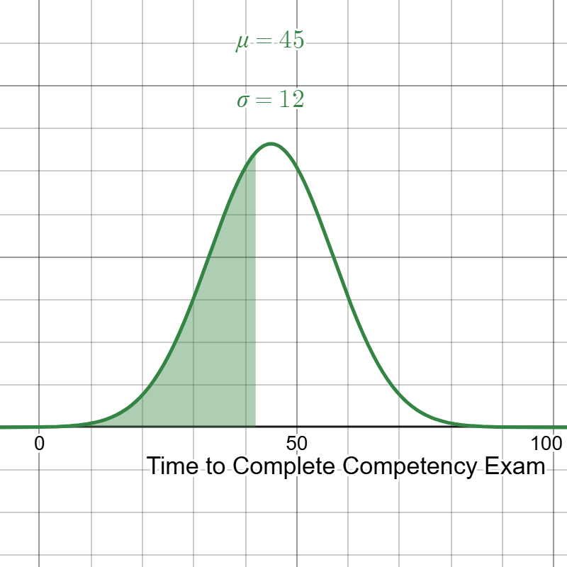
\(z = \frac{42-45}{12} = \frac{-3}{12} = -0.25\) \(P(t \le 42) = P(z \le -0.25) = 0.401 = \mathbf{40.1\%}\)

Now, instead of looking at just one student, you’re going to sample 30 students. Because of this, we expect a higher probability the average is closer to the mean, and a lower probability of an extreme value.

• What is the probability that the average time for your sample of 50 students is less than 42 minutes?

\[\mu_{\bar{x}} = \mu = 45 \qquad \sigma_{\bar{x}} = \frac{\sigma}{\sqrt{n}} = \frac{12}{\sqrt{30}} = \frac{12}{5.477} = 2.191\]

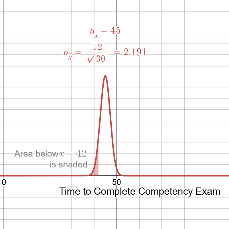
\(z = \frac{42-45}{2.191} = \frac{-3}{2.191} = -1.369\) \(P(t \le 42) = P(z \le -1.369) = 0.085 = \mathbf{8.5\%}\)

So, we see a much higher probability for a single individual, but a much lower probability for a group average.

Practice

Below are three problems regarding sampling distributions. Work on these problems, then click on the link to get the answer.

Practice Problem 1

The average commute time for workers in a large metropolitan area is 35 minutes with a standard deviation of 8 minutes. A researcher takes a random sample of 64 workers.

1. What is the probability that the commute time of a single passenger is less than 33.5 minutes?
   • (After completing this on your own, check the solution here.)
2. What is the probability that the sample mean commute time is less than 33.5 minutes?
   • (After completing this on your own, check the solution here.)

Practice Problem 2

A factory produces light bulbs with a mean lifetime of 1,200 hours and a standard deviation of 100 hours. A quality control engineer selects a random sample of 36 bulbs.

1. What is the probability that the lifetime of a single bulb is greater than 1,225 hours?
   • (After completing this on your own, check the solution here.)
2. What is the probability that the sample mean lifetime of the 36 bulbs is greater than 1,225 hours?
   • (After completing this on your own, check the solution here.)

Practice Problem 3

A coffee shop claims that the average temperature of its freshly brewed coffee is 160°F with a standard deviation of 5°F. A health inspector randomly samples 41 cups of coffee.

1. What is the probability that the temperature of a single cup is between 158°F and 162°F?
   • (After completing this on your own, check the solution here.)
2. What is the probability that the sample mean temperature is between 158°F and 162°F?
   • (After completing this on your own, check the solution here.)

Technology

Calculations here use normal distributions, so refer by to the Technology section in Lesson 15 lecture pages.