MATH 1040 - Introduction to Statistics

Lesson 18.1 Critical Values

Reading

Reading sections are from the Introductory Statistics Textbook

• 4.2.3 Normal approximation for the sampling distribution of \(\bar{x}\) (pages 162-163)

Lesson

In order to understand the confidence interval, let’s create a scenario. This is the problem we will work on through this lesson:

American mental abilities are often measured by an IQ test. The IQ distribution is normal with a mean of 100 and a population standard deviation of 15.

A random sample of 40 Snow College students is taken and they have an average IQ of 106.3. What is the true average IQ of Snow College students?

We can’t find the exact value for the true average. The only way to do that is to measure the entire population. Instead, we will create a range of numbers called a confidence interval. This range gives us an idea of the location of the true average.

We are going to create an interval, which is a range of numbers in which the true mean is likely to be.

• If we have a wider interval, the true value is more likely to be in the interval (higher confidence in our answer)
• If we have a narrower interval, the true value is less likely to be in the interval (lower confidence in our answer)

We will use normal distributions to determine the width of our interval. However, as we saw in lesson 17 on the Central Limit Theorem, the sample must be large enough for the central limit theorem to apply. Namely,

• the sample must be random, and
• the sample must be large enough (\(n\ge 30\) for quantitative variables)

Now, consider a normal distribution with the central section selected. In the next figure, the central area of 90% is highlighted.

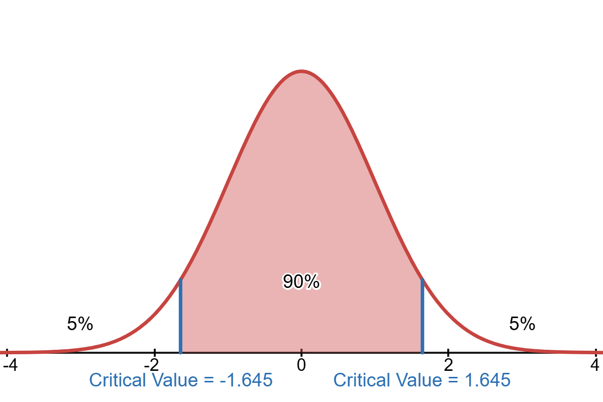
Since 90% of the area is in the center, the remaining 10% is in the tails (5% in the left and 5% in the right tail). Here are two ways to interpret this:

• We are 90% confident that the true value is in our interval (We have a confidence level of 90%)
• We accept a 10% chance that we could be wrong

What is the z-score that separates the tails from the center? If we take the left tail with an area of 5% (0.05), then you can look at this on a Z-Table or use a calculator to find a z-score of -1.645. Because the normal distribution is symmetric, we have a z-score of +1.645 on the right tail.

The critical value is the z-score that separates the central area from the tail(s) in a normal distribution.

So, the critical value of a 90% confidence level is \(\pm 1.645\).

Let’s consider now a confidence level of 95%. Here is a figure of the normal distribution with 95% of the area in the center and the remaining 5% in the tails (2.5% in each tail).

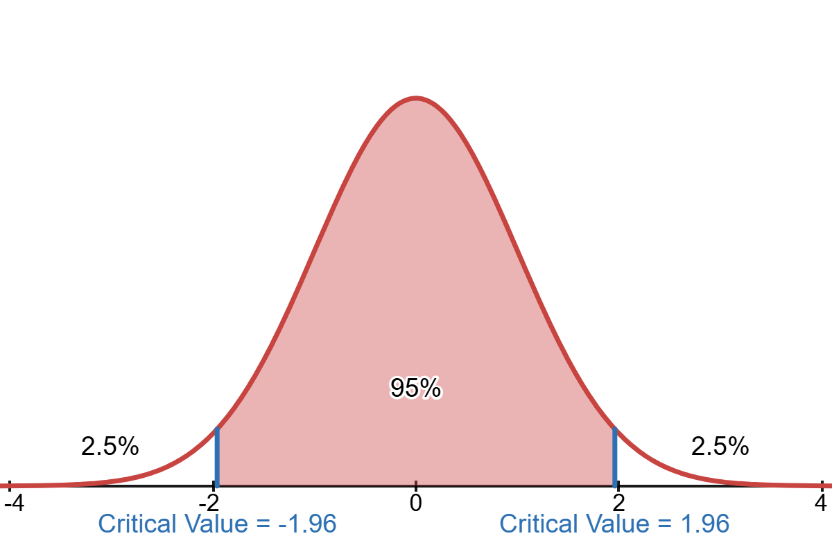
• We are 95% confident that the true value is in our interval (We have a 95% confidence level)
• We accept a 5% chance that we could be wrong

The z-score separating the left tail with an area 2.5% (0.025) from the center is -1.96. Because of symmetry, the z-score that separates the 2.5% in the right tail from the center is +1.96. So, the critical value of a 95% confidence level is \(\pm 1.96\).

Notice that the width (or range of values) of an area of 95% is wider than in an area of 90%. This is what we expect. With a wider interval, we have more confidence that the interval will contain our true value.

One more with an even wider interval. We’ll look at a confidence level of 99% with the remaining 1% in the tails (0.5% in each tail).

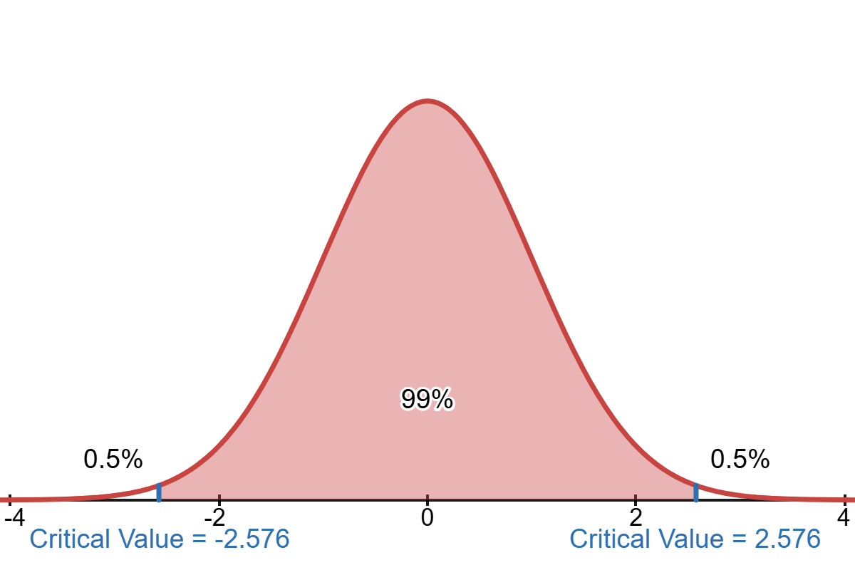
• We are 99% confident that the true value is in our interval (We have a 99% confidence level)
• We accept a 1% chance that we could be wrong

The z-score separating the left tail with an area 0.5% (0.005) from the center is -2.58. Because of symmetry, the z-score that separates the 0.5% in the right tail from the center is +2.58. So, the critical value of a 95% confidence level is \(\pm 2.58\).

We have just found the three most common critical values.

Confidence Level	Critical Value
90%	\(\pm 1.645\)
95%	\(\pm 1.96\)
99%	\(\pm 2.58\)

Other confidence levels are used, but these three are most common.

Practice

1. What is the critical value for the 76% confidence level?
   • After solving on your own, see solution here
2. What is the critical value for the 83% confidence level?
   • After solving on your own, see solution here
3. What is the critical value for the 92% confidence level?
   • After solving on your own, see solution here

Technology

TI-83/84

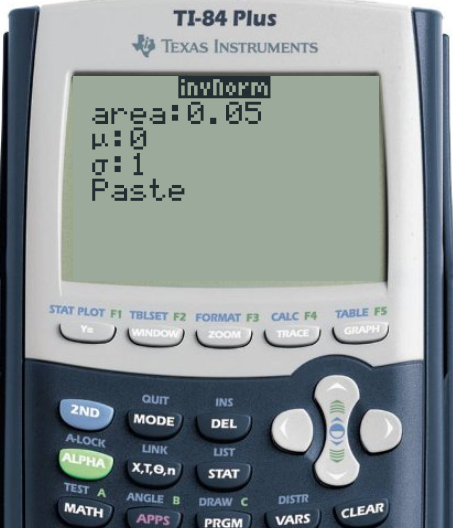
To determine the critical value, find the area of the left tail.

• For a 90% confidence level, the remaining 10% is in the two tails, 5% in each

On the TI-83/84,

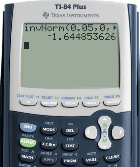
• 2nd [DISTR] –> 3:InvNorm(
• Type area, 0 (standardized mean), and 1 (standardized standard deviation)
• Press Enter

On the TI-84, you’ll see the first image. On the TI-83, you’ll go straight to the second image.

Desmos

To determine the critical value, find the area of the left tail.

• For a 90% confidence level, the remaining 10% is in the two tails, 5% in each

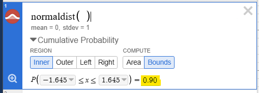
In Desmos,

• type normaldist() in one cell
  • Optional: Click the magnifying glass in the small panel left of the cell to view the full normal distribution
• Click the arrow next to “Cumulative Probability”
• Select the REGION as “Inner”
• Select the COMPUTE as “Bounds”
• After the $$P(\dots \le x \le \dots) = $$ line, there is a space to type your confidence interval

After doing this, the spaces in the \(P(\dots \le x \le \dots)\) will auto-fill with the critical values.

Note: You can also find the critical value using the area from the tail. Just select the Left or Right region and enter the tail’s area. This will be useful when we discuss Hypothesis Testing.