math3080
Statistical Learning
Reading
- James et al., Chapter 2
What is Statistical Learning?
This is an umbrella term for all statistical algorithms used to learn from data
- aka Data Mining
- aka Machine Learning
- algorithms aka models
Notation
Some common notation:
- $y$ is used for true output values
- $\hat{y}$ is used for predicted output values from a model
- $\vec{x}$ is a vector, or a series of values, such as input for a model
- $\mathbf{A}$ is a matrix, or a series of vectors, like a dataset or a series of observations - similar to the DataFrame or more like the 2D numpy array we have already seen
- $x_{ij}$ is the $j^{th}$ variable (column) of the $i^{th}$ observation (row) in a dataset (matrix)
Other notation can be given as we go along.
How Statistical Learning Works
Let’s consider a study comparing Years of Education to a person’s Income.
Draw a series of points that are almost sigmoidal with noise
In truth, there may be a relationship between the years of education and the income. This relationship is $f(x)$.
Draw $f(x)$ with a light grey color
However, no value exactly follows this relationship, so the true equation is,
\[y = f(x) + \epsilon\]where $\epsilon$ is a random error term. These errors come from outside influences that we have no control over, known as confounding variables. The function $f(x)$ that the data follows is truth.
In reality, though, we usually don’t know $f(x)$. We often have no way of knowing if there even is a true relationship. So, we are left to analyze (like we did using the tools we learned before Spring Break) and to create models to try to follow statistical patterns to estimate $f(x)$. This estimate is now $\hat{f}(x)$.
Draw $\hat{f}(x)$ somewhat off of $f(x)$
Since we have no way of estimating $\epsilon$, this is the best we can often do, so,
\[\hat{y} = \hat{f}(x)\]Statistical Error
Can we improve $\hat{f}(x)$? Absolutely! We do this by adjusting the settings of $\hat{f}(x)$ (known as parameters) little by little. By making little adjustments, we can be sure to help $\hat{f(x)})$ approach $f(x)$ as closely as possible.
How close can we get? There are two error quantities involved in this prediction:
- Reducible error: The part of the error we can minimize as we bring $\hat{f}(x)$ closer to $f(x)$
- Irreducible error: The part of the error we can’t reduce because of the noise (random error term $\epsilon$)
To explain this mathematically, we can find the expected value of the squared difference between the predicted and true values of y.
\[\begin{align*}E(y-\hat{y})^2 &= E[f(x) + \epsilon - \hat{f}(x)]^2 \\ &= [f(x) - \hat{f}(x)]^2 + var(\epsilon)\end{align*}\]The term $[f(x) - \hat{f}(x)]^2$ represents the reducible error as we can minimize this difference as the model improves. However, the random errors in $var(\epsilon)$ can never be reduced.
As a result, there will always be an upper bound on our accuracy metrics. If we ever get a 100% accuracy measurement on our models, we should be very suspicious…
Overfitting
We can make $\hat{f}(x)$ fit $f(x)$ perfectly with high-degree polynomials
Graph a scatterplot with a high-degree polynomial hitting every single point and another graph showing the error of our model going down as the degree of our model goes up
However, if we introduce a new dataset that this model hasn’t seen before, we’ll see the error drop to a point. But once the model reaches a degree high enough that it starts being taylored to the training data, the errors for this new dataset will go up.
Add errors for the new dataset to the error graph
How do we prevent this? We use a method called cross validation. We take our dataset and set aside 20-40% of our data in reserve for testing. We use the remaining 60-80% of our data to train our model. Once our model is trained, we check the performance of our model with our test data.
Now what is the problem with overfitting? Why not try to catch all the points in our training data?
- The job of $\hat{f}(x)$ is to try to model $f(x)$
- When overfitting $\hat{f}(x)$, we are also trying to model $\epsilon$, but since $\epsilon$ is just random error, that means we are trying to model randomness which is impossible
Basically, overfitting is trying to reduce the irreducible error.
Models vs. Inference
In one of our first lectures, we learned that there are three stages to Data Science, and we used an astronomical example for this:
- Gathering data (Tico Bray collected data on planetary motion)
- Analysis and Modeling (Johannes Kepler created equations that seemed to explain planetary motion)
- Explanation and Generalization (Isaac Newton created the Law of Universal Gravitation which gave meaning to Kepler’s equation and explained planetary motion)
Let’s revisit this in light of what we have learned about Statistical Learning.
When we are modeling, our goal is to find the value of $\hat{y}$, but the function $\hat{f}(\vec{x})$ is ultimately not important. (This was Kepler’s job in the astronomy example.)
- In some cases, this function is unknown - a black box.
- In fact, some argue that Neural Networks shouldn’t be used at all because even though we know the number that make the model $\hat{f}(\vec{x})$, we really don’t have any meaning to those numbers
However, when we are doing Inference, our goal is not necessarily to find the value of $\hat{y}$, but to understand and estimate $f(x)$ itself. (This was Newton’s job in the astronomy example.)
Our plan from here
- What are supervised models?
- Models with labels (pictures of cats, dogs, cows, goats, etc.)
- What are unsupervised models?
- Where should we build 5 franchises of our store given the distribution of a bunch of cities?
Quantitative vs. Categorical Models
These are a list of some of the common models that we will be seeing through this semester and the next:
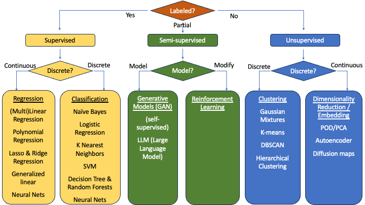
We’ll learn most of these models throughout the three semesters. This semester, I hope to show one model:
- Regression (Quantitative Supervised model): Linear Regression
- Classification (Categorical Supervised model): Logistic Regression
- Clustering (Categorical Unsupervised model): Hierarchical Clustering